07. Statistics(ANOVA)

[toc]

석회황이 벌에게 미치는 효과 분산분석 보고서

R의 OrchardSprays는 8가지 농도(A > B > ... > H)의 석회황유화액(lime surphur emulsion)을 자당 용액(sucrose solution)에 섞은 후, 농도별로 8개의 벌 방에 발랐다. 여기에 100마리 벌을 넣은 후 2시간 뒤, 각 벌 방에서 줄어든 자당 용액의 양을 측정하였다.

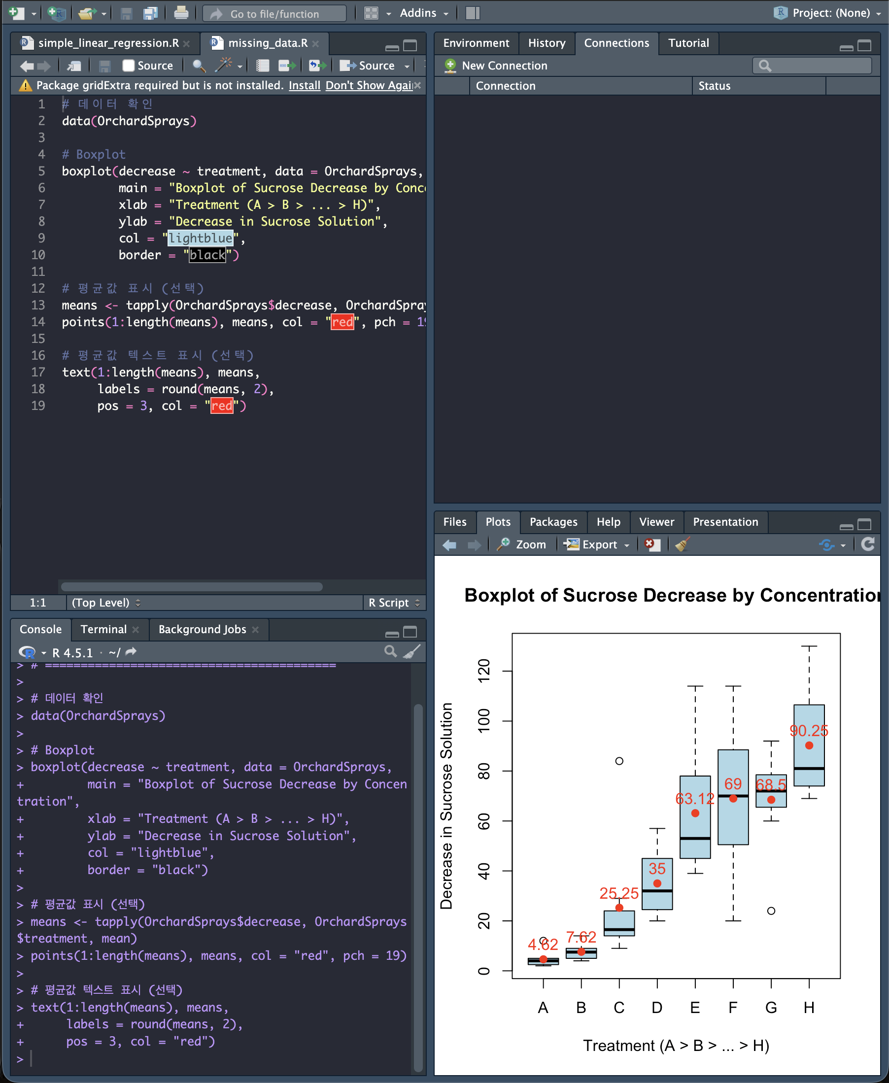
그림 1은 농도별 자당 감소량의 상자도표(boxplot)이며, 표 1은 각 농도별 자당 감소량의 평균과 표준편차 등을 요약한 기술통계 표이다.

또한 일원분산분석(ANOVA)을 이용하여 석회황 농도에 따라 자당 감소량이 유의미하게 달라지는지를 확인하고, 사후 분석으로 던컨의 다중비교법(여기서는 Tukey HSD 대체)을 사용하여 농도 간 차이를 비교하였다. 유의수준은 0.05로 설정하였다.

---

농도별 자당 감소량 boxplot

# 데이터 확인
data(OrchardSprays)

# Boxplot
boxplot(decrease ~ treatment, data = OrchardSprays,
        main = "Boxplot of Sucrose Decrease by Concentration",
        xlab = "Treatment (A > B > ... > H)",
        ylab = "Decrease in Sucrose Solution",
        col = "lightblue",
        border = "black")

# 평균값 표시
means <- tapply(OrchardSprays$decrease, OrchardSprays$treatment, mean)
points(1:length(means), means, col = "red", pch = 19)

# 평균값 텍스트 표시
text(1:length(means), means,
     labels = round(means, 2),
     pos = 3, col = "red")

---

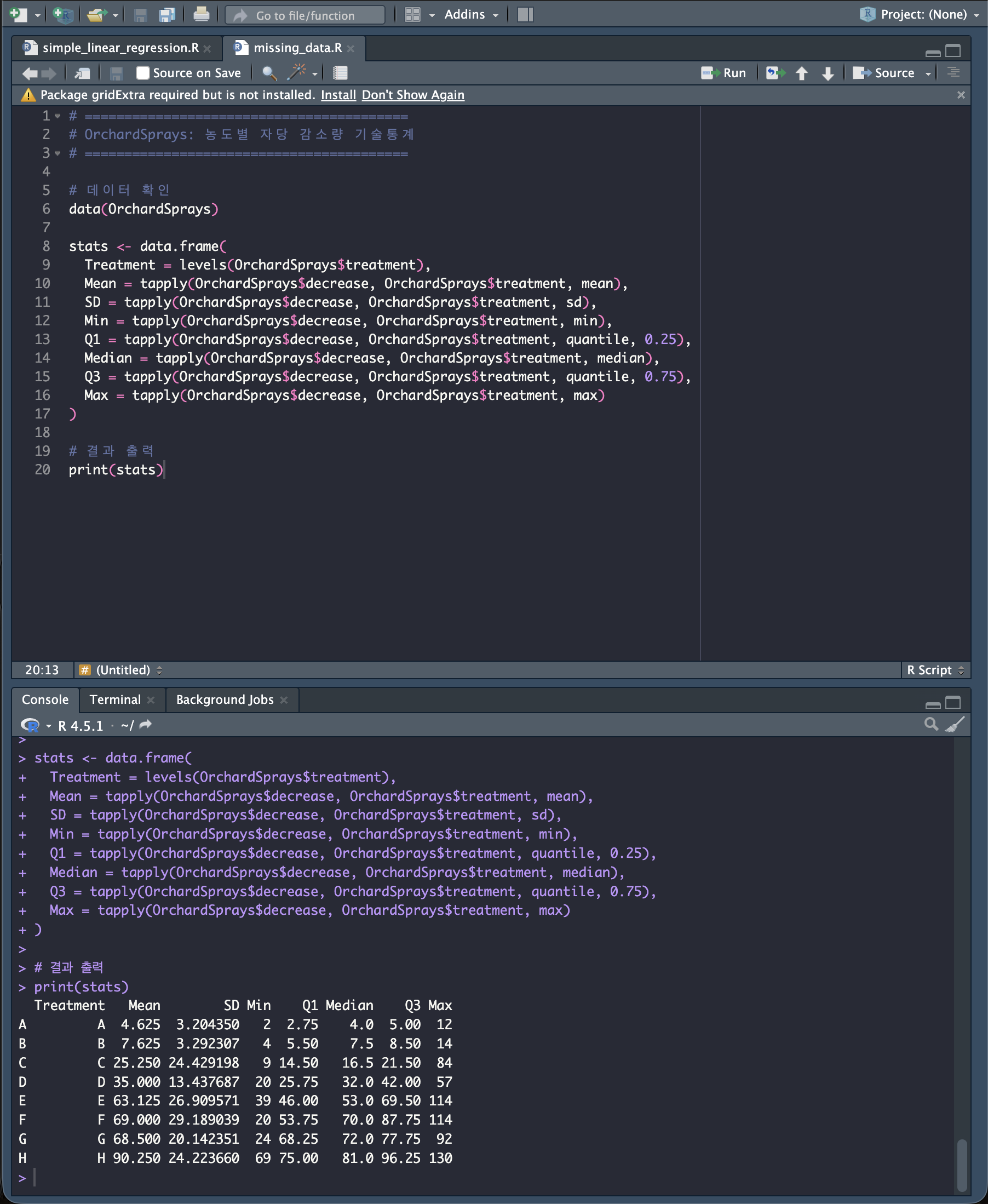
석회황 농도별 자당 감소액의 기술통계

# 데이터 확인
data(OrchardSprays)

stats <- data.frame(
  Treatment = levels(OrchardSprays$treatment),
  Mean = tapply(OrchardSprays$decrease, OrchardSprays$treatment, mean),
  SD = tapply(OrchardSprays$decrease, OrchardSprays$treatment, sd),
  Min = tapply(OrchardSprays$decrease, OrchardSprays$treatment, min),
  Q1 = tapply(OrchardSprays$decrease, OrchardSprays$treatment, quantile, 0.25),
  Median = tapply(OrchardSprays$decrease, OrchardSprays$treatment, median),
  Q3 = tapply(OrchardSprays$decrease, OrchardSprays$treatment, quantile, 0.75),
  Max = tapply(OrchardSprays$decrease, OrchardSprays$treatment, max)
)

# 결과 출력
print(stats)

농도	평균	표준편차	반복수	최소	최대
A	4.625	3.204	8	2	12
B	7.625	3.292	8	4	14
C	25.250	24.429	8	9	84
D	35.000	13.438	8	20	57
E	63.125	26.910	8	39	114
F	69.000	29.189	8	20	114
G	68.500	20.142	8	24	92
H	90.250	24.224	8	69	130

---

일원분산분석 결과 (ANOVA Table)

# =========================================
# OrchardSprays: 일원분산분석 (ANOVA Table)
# =========================================

# 데이터 불러오기
data(OrchardSprays)

# 일원분산분석 모형 적합
fit <- aov(decrease ~ treatment, data = OrchardSprays)

# ANOVA Table 출력
anova(fit)

# 또는 (동일 결과)
summary(fit)

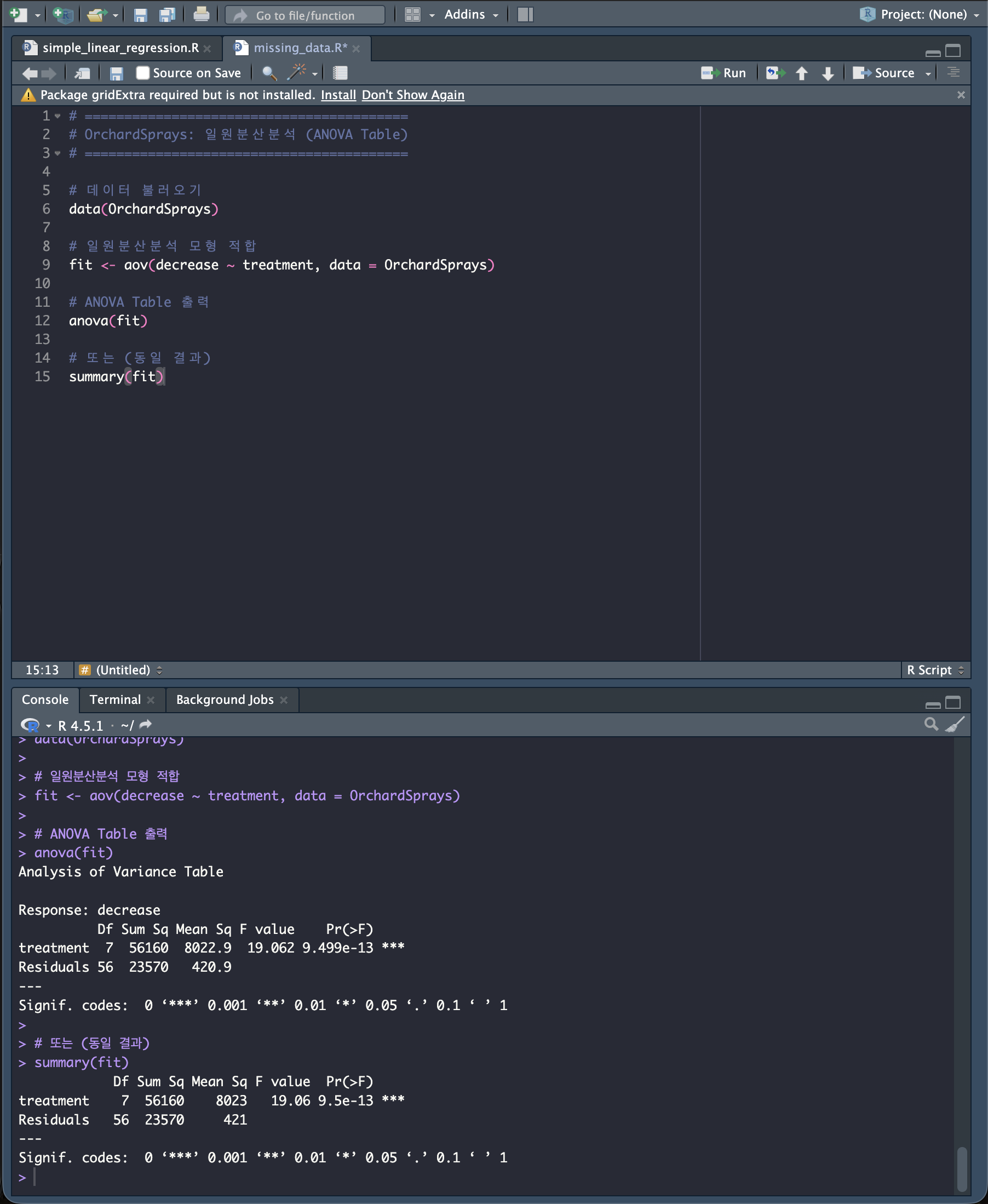
• 유의확률 p = 9.499e-13 이므로, 농도에 따른 자당 감소 효과는 동일하지 않다 (통계적으로 유의미한 차이가 존재).

---

던컨 다중비교 (Tukey HSD 결과)

# =========================================
# 그림 3: 던컨 다중비교 (Tukey HSD 대체)
# =========================================

# 데이터 불러오기
data(OrchardSprays)

fit <- aov(decrease ~ treatment, data = OrchardSprays)

tukey_result <- TukeyHSD(fit)

# 그래프
plot(tukey_result)

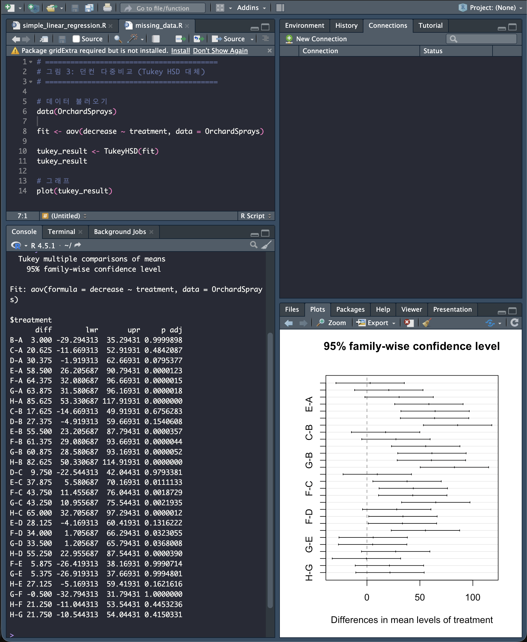
• Tukey HSD 결과에 따르면:
  • 농도 F, G, E는 동일 그룹으로 묶인다.
  • 농도 A, B는 동일 그룹이며 가장 감소량이 작다.
  • 농도 H는 유의하게 가장 높은 감소량을 보인다.

---

부록

Boxplot 코드

boxplot(decrease ~ treatment, data = OrchardSprays)

---

ANOVA 수행 코드

fit <- lm(decrease ~ treatment, data = OrchardSprays)
anova(fit)

ANOVA 콘솔 출력

Analysis of Variance Table

Response: decrease
          Df Sum Sq Mean Sq F value    Pr(>F)    
treatment  7  56160  8022.9  19.062 9.499e-13 ***
Residuals 56  23570   420.9                      
---
Signif. codes:  0 ‘***’ 0.001 ‘**’ 0.01 ‘*’ 0.05 ‘.’ 0.1 ‘ ’ 1

---

Duncan 다중비교 (Tukey HSD 대체) 코드

install.packages("agricolae")
library(agricolae)
duncan.test(fit, "treatment", alpha = 0.05, console = TRUE)

Duncan 다중비교 콘솔 출력 요약((Tukey HSD 결과)

  decrease groups
H   90.250      a
F   69.000      b
G   68.500      b
E   63.125      b
D   35.000      c
C   25.250     cd
B    7.625      d
A    4.625      d

---

End.